2D Light Field

The 2-dimensional light field data types provide a more convenient way to represent the light field in the plane space and can be used with our optical propagation methods.

OpticalPropagation.MonoLightField2D — Type

MonoLightField2D

MonoLightField2D is used to represent a 2-dimensional monochromatic light field.

MonoLightField2D(data; wavelength, size, center=(0u"m", 0u"m"))

size is the physical window width, while Base.size gives the sample counts. center is the centre of that window, not the mean of the sample coordinates. Dimension 1 is x and dimension 2 is y. Samples start at center - size/2, with pitches size ./ Base.size(data); the upper window endpoint is excluded. The public constructors copy the amplitude data into a Matrix{ComplexF64}.

Examples

julia> using Unitful

julia> MonoLightField2D([1 2; 3 4],wavelength=632.8u"nm",size=(1u"mm",1u"mm"))
MonoLightField2D:
    wavelength: 6.328e-7 m
    physical size: (0.001 m, 0.001 m)
    complex amplitude data:
2×2 Matrix{ComplexF64}:
 1.0+0.0im  2.0+0.0im
 3.0+0.0im  4.0+0.0im

source

Physical coordinates

The first array dimension is x and the second is y. size(field) gives sample counts; the existing field.size property and physicalsize(field) give physical window widths. gridcenter(field) is the window centre, which defaults to zero. It is not the arithmetic mean of the sample positions. For each dimension,

\[\Delta x = L_x/N_x, \qquad x_i = c_x - L_x/2 + (i-1)\Delta x.\]

This preserves the original half-open window convention, including odd sample counts and singleton dimensions. Coordinate ranges carry length units and use constant storage. axes(field) continues to provide integer array indices.

using OpticalPropagation, Unitful

field = MonoLightField2D(ones(4, 3),
    wavelength=633u"nm", size=(8u"mm", 6u"mm"),
    center=(10u"mm", -3u"mm"))
samplepitch(field)

(0.002 m, 0.002 m)

x, y = coordinates(field)
collect(x), collect(y)

(Unitful.Quantity{Float64, 𝐋, Unitful.FreeUnits{(m,), 𝐋, nothing}}[0.006 m, 0.008 m, 0.01 m, 0.012 m], Unitful.Quantity{Float64, 𝐋, Unitful.FreeUnits{(m,), 𝐋, nothing}}[-0.006 m, -0.004 m, -0.002 m])

Existing constructors still work without center. The copy constructor inherits the centre unless it is explicitly changed. Replacing size changes the window widths around that centre; replacing data with a different matrix shape keeps the same window and changes the sampling pitches. These operations relabel the samples; they do not interpolate or resample the amplitude. Public constructors and copy(field) make independent amplitude matrices.

crop(field, I, J) instead extracts a rectangular region while preserving its physical sample positions and pitches. It accepts nonempty contiguous unit ranges and : and copies the selected data. Ordinary array slicing retains its existing behaviour and returns data without light-field metadata.

region = crop(field, 2:3, 2:3)
physicalsize(region), gridcenter(region), coordinates(region)

((0.004 m, 0.004 m), (0.01 m, -0.002 m), ((0.008:0.002:0.01) m, (-0.004:0.002:-0.002) m))

Scalar arithmetic and same-grid broadcasting preserve coordinates. Combining light fields checks sample counts, wavelength, physical widths and window centres, including in-place assignments. Centre differences are compared at the sample pitch scale, so a large absolute centre does not hide a displacement of one pixel. Unlabelled matrices and vectors can be used as masks with ordinary broadcasting rules, provided they do not expand the physical grid. No interpolation or coordinate alignment is performed implicitly.

parent(field) returns the actual Matrix{ComplexF64} without copying. Use this for matrix FFTs and plans; such operations return numerical data and do not construct frequency-coordinate metadata. Mutating the parent also mutates the light field.

OpticalPropagation.physicalsize — Function

physicalsize(light::MonoLightField2D)

Return the physical window widths (Lx, Ly), also available as light.size. A width is the sample count times the pitch, not the distance between endpoints.

source

OpticalPropagation.samplepitch — Function

samplepitch(light::MonoLightField2D)

Return the sampling pitches (Δx, Δy) with length units. Empty dimensions have no defined pitch and cause an ArgumentError.

source

OpticalPropagation.gridcenter — Function

gridcenter(light::MonoLightField2D)

Return the physical window centre (cx, cy). This is not the mean of the sample coordinates, which lie in a half-open window.

source

OpticalPropagation.coordinates — Function

coordinates(light::MonoLightField2D)
coordinates(light::MonoLightField2D, dim)

Return unitful coordinate ranges (x, y), or the range for dimension 1 or 2. Ranges use constant storage and start at gridcenter(light) - physicalsize(light)/2. Base.axes(light) continues to return ordinary integer indices.

source

OpticalPropagation.crop — Function

crop(light::MonoLightField2D, I, J)

Copy a nonempty rectangular region into a new light field, preserving its wavelength, sampling pitches and physical sample positions. I and J must be contiguous integer unit ranges or :. Ordinary indexing retains Julia's array behaviour and does not attach physical coordinates to slices.

source

Work with Plots.jl

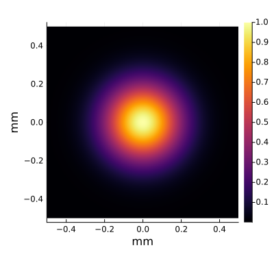
The 2-dimensional light field data types can work with Plots.jl, so it will be more convenient when we want to visualize a light field. For example,

using Unitful
using Plots

gauss = MonoLightField2D(
    [exp(-(x^2+y^2)/6400) for x in -200:199, y in -200:199],
    wavelength=632.8u"nm",
    size=(1u"mm", 1u"mm")
)
plot(gauss)